CAPM stands for Constant Acceleration Particle Models, wherein we built from our former understanding to develop a knowledge and appreciation of what constant acceleration means.
This added acceleration graphs to our chart in contrast with velocity, showing how they intermingled. Then we worked on how we could translate from a motion graph, to a velocity graph, and then to one for acceleration.
CAPM.1
Instantaneous velocity:
This is the velocity at any precise, given, point in time. It can be calculated in several ways from either charts or graphs. If at a graph, one can tell the velocity by using exactly where it is on a v vs t graph, such as the one below that is both constant velocity and constant acceleration.
Thus, by finding the exact position of an object which is its data points on a v vs t graph, we can see what the exact instantaneous velocity is.
 |
| http://www.thetrc.org/pda_content/texasphysics/e-BookData/Images/SB/57/LR/ConstAccelConstVelComparisons.png |
Thus, by finding the exact position of an object which is its data points on a v vs t graph, we can see what the exact instantaneous velocity is.
The second way to solve for velocity is by taking mirroring in time data points on both sides of what you are looking for, and then inputting them into the formula V= Change in position/ Change in time.
Capm.2
Solving for displacement can be solved for either with formula's or with a graph.
The formula is Change in x= xfinal-Xinitial on a x vs t graph, however on a velocity vs time graph the formula becomes change in x= 1/2*a(change in t)^2+ Vi(total time)
On a graph, we can use the position vs time graph to see where it is by subtracting the initial data points from the final coordinates.
Capm.3
Solving for acceleration can be done in four ways.
The first is looking at a velocity vs time graph, where we can input our data into the formula a=Change in v/ change in t.
The second is solving for it in other formula's, such as solving for a in the following formula Change in x= 1/2 a (change in t)^2 + Vit.
The third is simply looking at an acceleration vs time graph and seeing where it is.
The fourth is solving for it in the second formula:
Vf=a(change in time)+V(initial)
CAPM.4
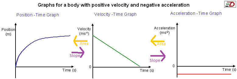
If you look at the following position vs time graph, you may note:
 |
| This is taken from http://gradeelevenphysics.weebly.com/speed-velocity-and-acceleration.html |
You may note that it is constantly decreasing its velocity, however the acceleration is constant. It is travelling in a positive direction though the velocity and acceleration are negative as it is slowing down.
The corresponding v vs t graph would resemble the one above, with it constantly decreasing. The acceleration is steady but nonetheless negative as it is slowing.
CAPM.5
If we take the same graph as above, we can draw a position vs time graph based on our initial understanding of what the motion means. Because our velocity vs time graph is starting positive, and never becomes negative, we know that our position vs time graph will be positive. We also know that initially it will be going faster, as our velocity graph starts from a higher position on the y (Velocity) axis. Then, as our velocity slopes downward, we know that our position vs time graph line needs to lessen its upward motion, gradually curving out until it is almost going straight.
Due to the constant nature of our velocity going towards the x (time) axis, we know that it is heading in a negative direction and thus our acceleration will be negative and a straight line.
CAPM.6
In order to construct a graph, we must see that there are 4 particles.
The 4 particles are:
What direction is it going?
Is it constant?
What variables are we given, and what do they apply to?
Is it possible for it to become negative?
From this, we can draw any graph we wish.
CAPM.7
To solve for time, we can take the average formula x=1/2 a(t^2)+Vi(total time).
From this, we can solve using algebra to isolate our t.
Please note the image below to see the process.

No comments:
Post a Comment